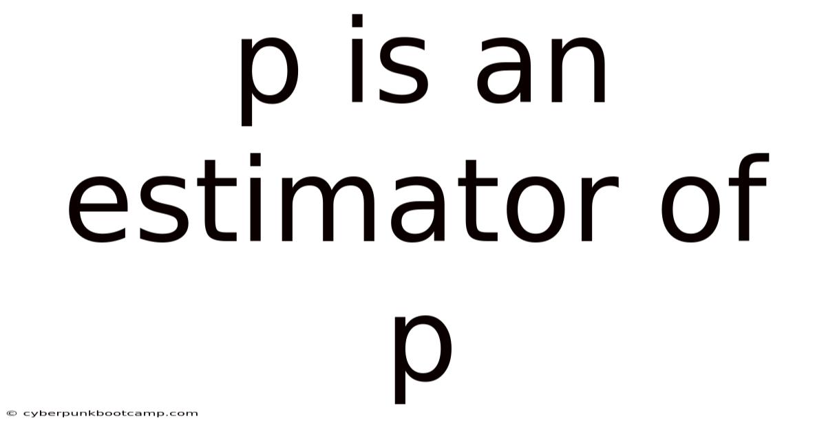
In statistics, the statement “p is an estimator of p” is a shorthand way of expressing that the sample proportion, usually written as (\hat{p}), serves as an estimator for the true population proportion (p). Understanding why (\hat{p}) works, how it behaves, and what assumptions underlie its use is essential for anyone designing surveys, analyzing experimental data, or interpreting poll results. This concept lies at the heart of inferential statistics, where we use information from a subset of individuals to make conclusions about an entire population. The following sections break down the idea step by step, provide a scientific explanation of its properties, and answer common questions that arise when applying this estimator in practice.
Introduction
When researchers want to know the proportion of a population that possesses a certain characteristic—such as the percentage of voters who favor a particular candidate, the share of defective items on a production line, or the prevalence of a disease in a community—they rarely can examine every single member. The sample proportion (\hat{p}) is therefore called an estimator of (p). Instead, they draw a random sample, compute the proportion of successes within that sample, and treat that value as an estimate of the unknown population proportion. The phrase “p is an estimator of p” simply reminds us that the symbol we use for the estimate ((\hat{p})) is derived from the same letter that represents the parameter we wish to learn about ((p)) Worth keeping that in mind..
Understanding Population Proportion and Sample Proportion
Population proportion ((p))
The population proportion is a fixed but unknown value that describes the fraction of individuals in the entire population exhibiting the trait of interest. Formally, if (N) is the population size and (X) is the number of individuals with the trait, then
[ p = \frac{X}{N}. ]
Because (N) is often huge or infinite, (p) cannot be measured directly in most practical situations But it adds up..
Sample proportion ((\hat{p}))
A sample of size (n) is drawn (ideally) at random from the population. Let (x) be the number of successes observed in the sample. The sample proportion is
[ \hat{p} = \frac{x}{n}. ]
Although (\hat{p}) varies from sample to sample, its expected value equals the true population proportion, making it an unbiased estimator of (p). This property is the foundation for confidence intervals and hypothesis tests concerning proportions.
Steps to Compute (\hat{p}) and Examine Its Properties
- Define the characteristic of interest – Clearly state what counts as a “success” (e.g., voting yes, being defective, testing positive).
- Select a random sample – Use a probability‑based sampling method (simple random sampling, stratified sampling, etc.) to avoid bias.
- Count successes and sample size – Record (x) (number of successes) and (n) (total sampled units).
- Calculate the sample proportion – Compute (\hat{p}=x/n).
- Assess sampling variability – Recognize that (\hat{p}) is a random variable; its distribution depends on (n) and the true (p).
- Check conditions for normal approximation – For large (n), the sampling distribution of (\hat{p}) is approximately normal if (np \ge 5) and (n(1-p) \ge 5).
- Construct a confidence interval – Use (\hat{p} \pm z^{*}\sqrt{\frac{\hat{p}(1-\hat{p})}{n}}) for a desired confidence level.
- Perform hypothesis testing – Compare (\hat{p}) to a hypothesized value (p_{0}) using a z‑test statistic (z = \frac{\hat{p}-p_{0}}{\sqrt{p_{0}(1-p_{0})/n}}).
Following these steps ensures that the estimator (\hat{p}) is used correctly and that inferences drawn from it are reliable Small thing, real impact..
Scientific Explanation: Why (\hat{p}) Estimates (p)
Unbiasedness
The expectation of (\hat{p}) is
[ E(\hat{p}) = E!\left(\frac{x}{n}\right) = \frac{1}{n}E(x). ]
Since (x) follows a binomial distribution (\text{Bin}(n,p)), we have (E(x)=np). Substituting gives
[ E(\hat{p}) = \frac{np}{n} = p. ]
Thus, on average, the sample proportion hits the true population proportion; there is no systematic over‑ or under‑estimation Simple as that..
Variance and Standard Error
The variance of (\hat{p}) derives from the variance of the binomial count:
[ \operatorname{Var}(\hat{p}) = \operatorname{Var}!\left(\frac{x}{n}\right) = \frac{1}{n^{2}}\operatorname{Var}(x) = \frac{1}{n^{2}}np(1-p) = \frac{p(1-p)}{n}. ]
The standard error (SE) is (\sqrt{p(1-p)/n}). In practice, we substitute (\hat{p}) for (p) to estimate the SE from the observed data Which is the point..
Sampling Distribution and the Central Limit Theorem
For a fixed (p), the distribution of (x) is binomial. When (n) is sufficiently large, the Central Limit Theorem (CLT) tells us that the standardized variable
[ Z = \frac{\hat{p}-p}{\sqrt{p(1-p)/n}} ]
approaches a standard normal distribution. Because of this, (\hat{p}) itself is approximately normal with mean (p) and variance (p(1-p)/n). This normality underpins the construction of Wald confidence intervals and the validity of z‑tests for proportions.
Consistency
As the sample size (n) grows, the variance (\frac{p(1-p)}{n}) shrinks to zero. So, (\hat{p}) converges in probability to (p); the estimator is consistent. Larger samples yield estimates that are increasingly close to the true proportion Most people skip this — try not to..
When the Normal Approximation Breaks Down
Even though the Central Limit Theorem guarantees asymptotic normality, the Wald interval (\hat p \pm z^{*}\sqrt{\hat p(1-\hat p)/n}) can be surprisingly poor for modest sample sizes or when the true proportion lies near the boundaries 0 or 1. In those regimes the interval often has coverage far below the nominal level and can even produce limits outside ([0,1]). Practitioners therefore often turn to methods that are exact or at least more dependable to skewness.
Exact (Clopper–Pearson) Confidence Intervals
The Clopper–Pearson interval is derived from the binomial probability mass function and guarantees that the true coverage is at least the stated confidence level. For an observed count (x) out of (n) trials, the lower and upper bounds ((L,U)) satisfy
[ \Pr\bigl{X\le x-1\bigr}= \alpha/2 \quad\text{and}\quad \Pr\bigl{X\ge x+1\bigr}= \alpha/2, ]
where (X\sim\text{Bin}(n,p)). In practice the bounds are expressed using beta quantiles:
[ L = \mathrm{Beta}{\alpha/2}(x, n-x+1), \qquad U = \mathrm{Beta}{1-\alpha/2}(x+1, n-x). ]
Because the interval is constructed from the exact binomial distribution, it is conservative—its width is typically larger than that of approximate methods, especially when (n) is small The details matter here..
Improved Approximate Intervals
Several approximate intervals have been proposed to retain the simplicity of the Wald method while improving coverage:
-
Wilson score interval – solves the quadratic inequality
[ \frac{\hat p - p}{SE(p)} = z^{*}, ]
where (SE(p)=\sqrt{p(1-p)/n}). The resulting closed‑form expression is
[ \frac{\hat p + \frac{z^{2}}{2n} \pm z^{}\sqrt{\frac{\hat p(1-\hat p)}{n} + \frac{z^{*2}}{4n^{2}}}}{1 + \frac{z^{*2}}{n}}. ]
This interval stays within ([0,1]) and has coverage much closer to the nominal level for a wide range of (n) and (\hat p).
-
Agresti–Coull (add‑z) interval – adds (z^{*2}/2) successes and failures to the data before forming the Wald interval. The adjusted proportion
[ \tilde p = \frac{x + z^{*2}/2}{n + z^{*2
